Algorithmic State Machine (ASM)

An Algorithmic State Machine (ASM) is a graphical notation similar to a flow-chart, the main difference being that an ASM also includes timing information. This notation can be used to specify the operation of both the datapath and the control unit.

Essentially, the ASM is a state diagram where the states have internal structure described by a simple flow-chart like notation. The symbols used in the notation are states, decisions, and conditional outputs.

State

The entry-point of a state is represented graphically by a rectangle. The name of the state and possibly the binary code assigned to the state are written outside the rectangle. Inside the rectangle register transfer operations and outputs are given. Register transfers will happen at the next positive clock edge (assuming positive edge flip-flops are used). Outputs will be immediately set to 1. Any output not mentioned in a state will be set to 0.

The actual state comprises all of the symbols that are to be found on all paths coming from the rectangle up to the next rectangle on such a path.

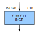
In the example below we have a state called INCR0 with binary code 010. There is a single register transfer which increments S and there is a single output called INCR.

Decision

A decision is represented graphically by a diamond (rhombus). The inside of the diamond contains the condition upon which the decision rests. Possible conditions could be checking the status of a signal, comparing two registers for equality, etc. Any such condition can have only one of two outcomes: 0 or 1. As the decision is made immediately, any register updated in the same state as the decision won't be seen by that decision during the current clock cycle.

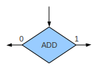
In the example below we have a decision which checks the signal ADD. What happens if ADD is 0 or 1 isn't shown.

Conditional Output

Conditional output is represented graphically by an oval. The inside of the oval contains the outputs to be set and register transfers to be made. The oval can only occur immediately after a decision. Note that if any outputs occur in an ASM oval, then that ASM describes a Mealy model. If no ovals exist, or no oval has an output, then we have a Moore model.

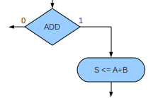
In the example below, we transfer the sum of A and B to S only when the signal ADD is 1.

Datapath Derivation

A well developed ASM contains all necessary detail to derive an appropriate datapath. We can see that any destination of register transfer will need to be a register, so we can analyse the ASM and build the set of registers needed. The register transfer operations performed will give us the combinational logic circuits needed, e.g., adder/subtractors, shifters, etc. It may be the case that the operations dictate that some registers will be best implemented as counters or shift registers. We also need to analyse the decisions found in the ASM as these may need circuits such as comparators.

Control Unit Derivation

As mentioned earlier, the ASM can be seen as a type of state diagram. We also know that a state diagram can be transformed into a state table, and that a state table can be used to derive a sequential logic circuit. To build a complete state table, we need all the input and output signals. We have all external input and output signals explicitly given in the ASM, and, after deriving the datapath we have can find the set of internal control signals and how they will need to be manipulated in each state, and this gives us what we need to complete state table.

Example

As an example of an ASM, consider the Euclidean greatest common divisor (gcd) which is one of the oldest algorithms we know of. Mathematically, the gcd of two positive integers is defined as follows:

gcd(a,a) = a
gcd(a,b) = gcd(a-b, b)    if a>b,
gcd(a,b) = gcd(a, b-a)    otherwise.
	

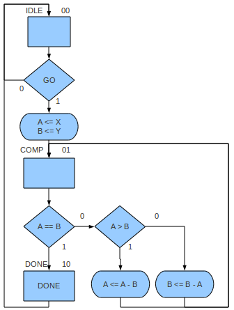
The following ASM was created to implement the gcd. It comprises three states (IDLE, COMP, and DONE), two registers (A and B), three inputs (X, Y, and GO), and two outputs (DONE and either A or B — let's choose A). If the initial state is IDLE and the arguments of the gcd are X and Y, then gcd(X,Y) will eventually be loaded into A. The input GO starts the whole process, and the output DONE is pulsed (0 to 1) when A contains the result.

References

Mano, M. Morris, and Kime, Charles R. Logic and Computer Design Fundamentals. 2nd Edition. Prentice Hall, 2000.